Using Geometric Financial Analysis to Determine True Fixed and Variable Behavior
Geometric Analysis
Time to drop the arbitrary labels and let the numbers speak. We accountants do our best to characterize expenses as variable or fixed based on the nature of the expense and its relationship to the business activity, but what if they don’t actually behave that way? Or, more deceptively, behave in a variable manner only at certain sales levels and fixed at others?
Who cares but you accountants? You should, if you care about the effectiveness of your pricing strategy, or the accuracy of your projected financial statements. Further, you cannot know your break even level of sales with an inaccurate picture of your fixed costs.
Understanding your actual variable and fixed cost behavior can also share revealing information about the productivity and efficiency of your business. Analyzing a specific expense or expense units (such as manufacturing labor) over a range of sales can show you the range of variability in that expense item and give you an indication of how to optimize the expense for maximum productivity within a sales range.
CASE STUDY: MANUFACTURING
In the following case study we will analyze a small manufacturing company’s profitability and cost behavior over a range of years, determine the actual variable and fixed cost levels, and develop an reliable financial model of the business that can accurately project the company’s profitability at any level of sales within a historical range.
Historically, this company’s profitability has ranged from 6-15% of sales, depending on the level of sales. Manufacturing overhead, that portion of overhead expenses assigned to Cost of Goods Sold was $5.6 million in 2013 when sales were $9.1 million. However, these expenses do not behave in a truly fixed manner and vary significantly with sales. In that same year the company had Operating Expenses of $2.2 million. These expenses also vary with sales, but to a much lesser extent. How can we determine the company’s true fixed costs and variable cost percentage based on its financial history? The table and graph below lists the company’s sales and profit over history.


In the following table, the sales and profit data have been resorted based on sales.

In the following graph, the resorted sales were plotted against the profit information, which produces a far more revealing graph.

If a line were created that passed evenly between the points on this graph, it would be an accurate representation of what we would generally expect the company’s profit to be at any given level of sales. The amount of fixed costs is documented by the Y-axis intercept point, which is approximately -1,500,000. This means that if sales (X-axis) were zero, the company would lose approximately $1,500,000. The slope of this line indicates the variable cost percentage of sales; 71% in this case.
In the following graph, we add a line with these characteristics, called Model. Note that this line passes through the point marking the nine-year averages of sales and profit.
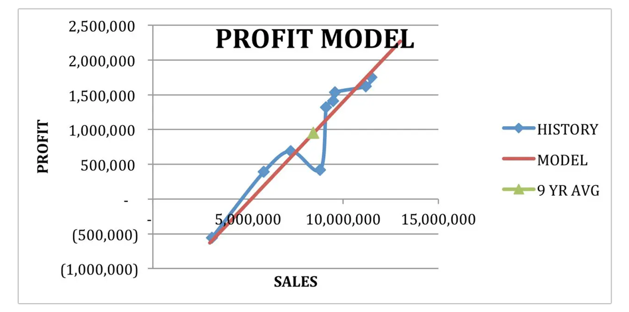
Which is a more accurate predictor of the future, the model of the company’s behavior or the historical results at any given level of sales? For example, in 2008 the company had approximately $8.8 million in sales but had a profit of just over $400K (causing the dip in the historical graph). Isn’t this actual history more reliable than the model, which suggests that the profit should have been over one million? The model will be a more accurate predictor of the future than the actual historical results in any given year. This is because every individual year’s results contain a number of financial anomalies and inconsistencies of varying magnitude, which will never be repeated. The model averages these inconsistencies out, offering the most probable profit outcome for any given level of sales.
Having an accurate predictor of profitability at every level of sales is a very important tool when a company is considering offering pricing incentives to reach a higher level of sales, or additional capital investment to increase capacity.
A similar analysis can be performed on an individual expense item to determine the fixed and variable attributes of that activity. Below is a table of the labor costs included in Cost of Goods Sold. This account is normally presumed to be 100% variable. Ideally, this account would be analyzed using operating data – labor hours – instead of the expense in dollars to factor out pricing differences over time. Because we do not have access to the labor hours data in this case, I have shortened the data range from nine years to six to reduce the effects of inflation.

The following table and graph display the same data, resorted by sales.

The six-year average labor cost as a percent of sales is 16.6%. However using our graph, we find that a graph with a Y-axis intercept of 75,000 (the fixed portion of labor spending) and a slope of 15.5% produces a line that passes through the historic average and represents the historic trend. Based on this model, we can forecast that increases in sales will actually increase labor costs by 15.5%, not by 16.6% as the historic average suggests.
Based on that information, labor costs as a percentage of sales will decline as sales increase within this range, however this will happen only slightly due to the relatively low fixed cost portion (75,000).


Brian Murray
Brian has been in public accounting since 1997. Prior to that he was in finance at Kimberly-Clark Corp., audit at M&I Bank Corp., and accounting manager at Browning-Ferris Ind. Brian’s areas of specialty are estate and trust tax and business valuation.